Back to the Introduction.

1.A - Tables and graphs of standard data

Rather than break up the main presentation, I collect here some samples of the kinds of reference data and graphs that are available for use in analyzing fluid drag problems.

This first table gives a few typical fluid paramaters. Note that this table uses the cgs units of Ref. [1].

	$\eta$	$\nu$	$\rho$
Water at 20 $^{\circ}{\rm C}$	1.005 x 10-2 g/(cm s)	1.007 x 10-2 cm2/s	$\approx$ 1 g/cm3
Air at 20 $^{\circ}{\rm C}$	1.808 x 10-4 g/(cm s)	0.150 cm2/s	$\approx$ 0.0013 g/cm3

Table:

Common values for the viscosity ($\eta$),
the kinematic viscosity ($\nu$), and
the density ($\rho$) of two familiar fluids.

C_D for a perfect sphere

Spheres have long been among the objects studied because of their ideal shape and common use as projectiles in the early history of ballistics. The data that lead to the red curve shown in the graph below are for a smooth sphere, and the curve used is a smooth line drawn through the data. The blue and green dashed lines are approximations that are discussed below.

Figure 1.1:

Graph, adapted from Ref. [1], of C_D versus Re for a sphere.

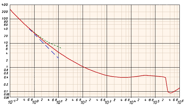
The blue dashed line shows the approximation due to Stokes' theory for fluid flow around a smooth sphere at very low Reynolds number. The formula obtained by Stokes says the drag force is linear in the speed v and predicts that C_D = 24/Re. The definitions used are that Re = vD/ $\nu$ and L² = $\pi R^2$, where D = 2R is the diameter of the sphere. (Notice that the 1/Re dependence produces a straight line on the semi-log plot above.) The graph shows that this approximation starts to break down even before Re = 1, so we can only assume a simple linear v-dependence for the drag on a smooth sphere for very small values of Re.

The green dashed curve shows an improvement to this expression due to Oseen, who obtained

$$C_D = \frac{24}{Re} \left( 1 + \frac{3}{16} Re \right)$$

for a correction to Stokes' expression. Empirically one notes that using a factor of about (1/12) instead of (3/16) would describe the data for values of Re close to 10 before starting to fail, but this expression for C_D does not have a simple velocity dependence so the results derived here will not apply to it. However, since it is a combination of linear and quadratic drag terms, it could be treated analytically if you had a good reason to.

Note that the red curve is approximately flat for Reynolds numbers between about 1000 and 300,000. In this region the drag force on a smooth sphere has a simple v² dependence.

C_D for a cylinder

Another case where there are data for drag on a simple object is that for a smooth cylinder transverse to the flow. I show an example of the drag coefficient for that case below. It shows many of the charateristics we saw in the case of the sphere.

Figure 1.2:

Graph, adapted from Ref. [1], of C_D versus Re for a cylinder.

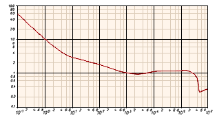
Although I will not discuss the case of the cylinder in any detail, it could make a good example for home-laboratory study and has its practical application in things like bridge supports in a river.