Back to the N=2 (Quadratic Drag) case

5. Sample Results

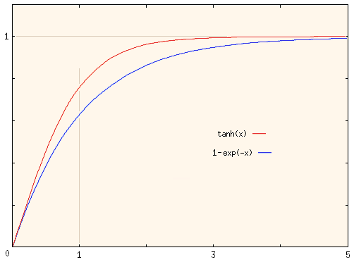
To illustrate the properties of these solutions, let us make some graphs of the N=1 and N=2 solutions, with unit time constant and the same terminal velocity, as a guide to identifying them and possibly fitting data. The two results are:

Linear drag: The velocity for the N=1 case was given in Eq. (7) [in Section 3]:

$$v(t) \; = \; V_{\rm max} \left[ 1 - e^{-t/T_1} \right]$$

where T₁ [defined in Section 3] is the time constant for the "decay" of the velocity as it approaches the terminal velocity. This function is shown with the blue curve in the figure below for the V_max = 1 and T₁ = 1 case, which are effectively "natural" units that are easily scaled to any problem.

Quadratic drag: The velocity for the N=2 case was given in Eq. (10) [in Section 4]:

$$v(t) \; = \; V_{\rm max} \tanh(t/T_2)$$

where T₂ [defined in Section 4] is the time constant for the "decay" of the velocity as it approaches the terminal velocity. This function is shown below with the red curve and values of V_max = 1 and T₂ = 1, again effectively in "natural" units that are easily scaled to any problem.

Figure 5.1:

Plot of v(t) vs. t for the N=1 and N=2 solutions
with unit time constants and same terminal velocity.

Notice that the quadratic drag case (red curve) rises much more quickly and reaches the terminal velocity sooner. However, part of the difference you see is due to the fact that the time constants have different meaning for these two functions. They are not equal when t = 1 as we would wish if we were using the speed relative to the terminal velocity at t = 1 as a data point.

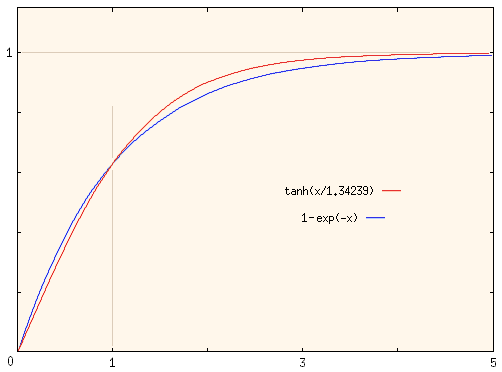
We can make the quadratic drag speed at t = 1 equal to that for linear drag (whose value is 0.63212 at t = 1) by choosing T₂ = 1.34239. This gives the result shown below.

Figure 5.2:

Plot of v(t) vs. t for the N=1 and N=2
solutions that have the same terminal
velocity and the same velocity at t = 1.

You can see that the velocity function for quadratic drag (red curve) still rises faster than that for linear drag, but the differences are not so dramatic. This shows that if you were to measure V_max and the time when v(t) reaches some intermediate value, you do not have enough information to choose between these two functions. Further, you can see that you need pretty good data at some other times to make that choice between models.

I say more about this in the next section.

Next, Fitting data to get C_D.