Back to the Sample Results.

6. Fitting data to get C_D

Fitting the equations to data is a non-linear least-squares problem. Since data for the velocity are, for most home-laboratory experiments, derived from position measurements, the experimental uncertainties of those velocity data are larger than your position estimates, which makes fitting more challenging. Note that you should use an expression like

$$v(\frac{t_1+t_2}{2}) \; \approx \; \frac{y(t_2) - y(t_1)}{t_2 - t_1}$$

to associate the average velocity over an interval with the time at the midpoint of the interval. This is only an approximation. It works best if the time intervals are as small as possible.

If you have a long enough data set that you see a terminal velocity, you get one parameter for free and the problem is much simpler. In that case you can then use one other data point to solve for the time constant in each equation. Then you can just compare all of the data to the two curves you get and choose the best one. Since neither is likely to be exactly right, you might have to try a few other time constants before you are happy. Plotting programs can make this much easier.

Acceleration data:

If you don't want to do a non-linear fit and the data do not give you a good handle on the terminal velocity, another alternative is to fit data for the acceleration on semi-log paper. You will, of course, have to calculate the acceleration date from the velocity data. [As with getting the velocity from change in position, the best approach is to associate the average acceleration over an interval with the time at the midpoint of the interval.] Note that the uncertainties in acceleration data derived from velocity data derived from position data will be large; however, they still might give you a better handle on whether the force you are dealing with is best modeled as linear or quadratic in v.

Acceleration for N=1

The acceleration for the N=1 case is obtained by taking the derivative of the v(t) determined in Section 3 [Eq. (7)] to get

$$a(t) \; = \; \frac{dv}{dt} \; = \; \frac{V_{\rm max}}{T_1} e^{-t/T_1} ,$$

where we note that V_max/T₁ = g, the acceleration of gravity. If we take the logarithm of each side, we get a straight line:

$$\log_{10} a(t) \; = \; \log_{10}\left[ \frac{dv}{dt} \right] \; = \; \log_{10}[g] \; - \; (0.4343) t/T_1.$$ (12)

Here I use the log base 10 (also used in the figure below), which is what introduces the factor of 0.4343. The intercept is just the log of g, while the slope is related to the (negative) inverse of the time constant, or just C. This means that plotting data for the acceleration on semi-log paper (or just plotting the log₁₀ of the data on regular paper) will give you the time constant, from which you can calculate the terminal velocity. A sample graph of Eq. (12) is shown with the blue line in the figure below.

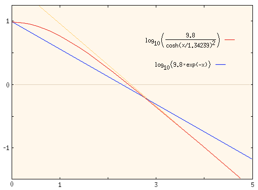
Note that the plot was made with g = 9.8 to be realistic for acceleration in metric units, but the unit time constant T₁ = 1 makes the slope totally arbitrary.

Figure 6.1:

Comparison of the log of the acceleration for the
N=1 (blue curve) and N=2 (red curve) cases similar
to those compared in the second graph of Section 5.

Acceleration for N=2

The acceleration for the N=2 case is obtained by differentiating the v(t) found in Section 4 [Eq. (10)] to get

$$a(t) \; = \; \frac{dv}{dt} \; = \; \frac{ V_{\rm max}/T_2 }{ \cosh^2(t/T_2) } \; ,$$

where we note that V_max/T₂ = g, the acceleration of gravity, and we have used that the hyperbolic secant is 1/cosh. If we take the log base 10 of each side we get result that looks messy, but actually has a simple structure:

$$\log_{10} a(t) \; = \; \log_{10}\left[ \frac{dv}{dt} \rig... ... = \; \log_{10}[g] - 2 \log_{10}\left[ \cosh(t/T_2) \right].$$ (13)

We can see that the zero intercept is just the lead constant, the log₁₀ of g, because

$$\cosh(x) \; = \; \frac{1}{2} \left( e^{x} + e^{-x} \right)$$

means that cosh(0) = 1 and the log of 1 is zero. Further, we can see that the cosh function is dominated by a single exponential at large t , giving a limit that we work out below. A graph of Eq. (13) is shown with the red curve in the figure above.

Note that I again use g = 9.8 to make the intercept realistic for values in metric units, and the time constant is T₂ = 1.34239, which was used for the second case considered in Section 5. Notice how an acceleration plot will amplify what seemed like subtle differences in the velocity graph. Since the uncertainties in the data you are fitting are also amplified, the fit might not be that much easier. Be careful.

Now consider what happens for large times (which corresponds to the approach to the terminal velocity). As t gets very large, we get

$$\frac{dv}{dt} \; \longrightarrow \; 4g e^{-t/T_2},$$

so the log of the acceleration becomes a straight line

$$\log_{10} \left[ \frac{dv}{dt} \right] \; \longrightarrow \; \log_{10} [4g] \; - \; (0.4343) t/T_2$$ (14)

in this large-t limit. This means that you can use a semi-log plot of data, or a plot of the base-10 log of the data, to identify the quadratic drag case from the shape of the curve, and extract the time constant from the slope at large times. [The graph above shows the asymptotic slope given by Eq. (14) with a light yellow line.] Once you know the time constant, you can deduce the terminal velocity and the function that should describe the velocity and position as a function of time. Estimating the slope of this curve at large t is an alternative to trying to guess the terminal velocity from a graph of v(t) that might be incomplete.

Final Comments:

Please note that the result of a fit using one of these two equations will only work properly if the drag is actually linear or quadratic in the velocity, not some arbitrary non-linear dependence on velocity that your are most likely to encounter in a real experiment. You may have to compromise and choose the better of two imperfect fits in order to maintain a simple model for the remainder of the analysis. You might have to obtain the best fit of each type from the acceleration data and then compare the corresponding velocity and position equations [Eq. (8) or Eq. (11)] to those data before making a choice of which looks best overall. The final test should always be to compare a graph of the equations you get to the data you actually measured (position or velocity) and see if it is acceptable.

The main advantage with the approach based on extracting and fitting the acceleration is that the shape of the graph early in the free-fall is indicative of which case the data favor. The main problem is that the uncertainties in the data increase as you derive accelerations from velocities from positions, and that these errors will likely be significant for larger times when the log of the acceleration is negative (i.e. when the acceleration is less than 1 m/s² in the plotted example). [Also note that the formulas I give are specific to using the base-10 log rather than the natural log.] In the end, a combination of methods and subjective judgements may be needed, as noted several times in this document.

A secondary advantage to deriving the acceleration is that you then have a graph that can be easily used to associate a force (from ma) at some particular time with the velocity at that same time, thereby constructing a force vs. speed graph that could be used in numerical calculations.

My final remark is to remember that you are working with real data. You will not get a perfect fit; your only goal is to get a reasonable fit and have some idea of the uncertainties in your proposed formula for the drag force. Plotting a family of curves, each with slightly different parameters, will show the sensitivity of your data to a variation in the parameters. Also remember that you can use your initial study to design a better calibration experiment, perhaps by trying to get better resolution data in some critical region. Your first experiment does not have to be your only experiment.

Return to the Overview